Teaching activity: Modelling complexity in industrial decarbonisation

Toolkit: Complex Systems Toolkit.

Author: James C Atuonwu, PhD, MIET, FHEA (NMITE).

Topic: Simulating pinch analysis and multi-stakeholder trade-offs.

Title: Modelling complexity in industrial decarbonisation.

Resource type: Teaching activity.

Relevant disciplines: Energy engineering; Chemical engineering; Process systems engineering; Mechanical engineering; Industrial engineering.

Keywords: Available soon.

Licensing: This work is licensed under a Creative Commons Attribution-ShareAlike 4.0 International License. It is based upon the author’s 2025 article “A Simulation Tool for Pinch Analysis and Heat Exchanger/Heat Pump Integration in Industrial Processes: Development and Application in Challenge-based Learning”. Education for Chemical Engineers 52, 141–150. 

Related INCOSE Competencies: Toolkit resources are designed to be applicable to any engineering discipline, but educators might find it useful to understand their alignment to competencies outlined by the International Council on Systems Engineering (INCOSE). The INCOSE Competency Framework provides a set of 37 competencies for Systems Engineering within a tailorable framework that provides guidance for practitioners and stakeholders to identify knowledge, skills, abilities and behaviours crucial to Systems Engineering effectiveness.   A free spreadsheet version of the framework can be downloaded.

This resource relates to the Systems Thinking, Systems Modelling and Analysis and Critical Thinking INCOSE competencies.

AHEP mapping: This resource addresses several of the themes from the UK’s Accreditation of Higher Education Programmes fourth edition (AHEP4):  Analytical Tools and Techniques (critical to the ability to model and solve problems), and Integrated / Systems Approach (essential to the solution of broadly-defined problems). In addition, this resource addresses the themes of Science, mathematics and engineering principles; Problem analysis; and Design. 

Educational level: Intermediate.

Educational aim: To equip learners with the ability to model, analyse, and optimise pathways for industrial decarbonisation through a complex-systems lens – integrating technical, economic, and policy dimensions – while linking factory-level design decisions to wider value-chain dynamics, multi-stakeholder trade-offs, and long-term sustainability impacts. 
 

 

Learning and teaching notes: 

This teaching activity explores heat integration for the decarbonisation of industrial processes through the lens of complex systems thinking, combining simulation, systems-level modelling, and reflective scenario analysis. It is especially useful in modules related to energy systems, process systems, or sustainability.  

Learners analyse a manufacturing site’s energy system using a custom-built simulation tool to explore the energy, cost and carbon-emission trade-offs of different heat-integration strategies. They also reflect on system feedback, stakeholder interests and real-world resilience using causal loop diagrams and role-played decision frameworks.  

This activity frames industrial heat integration as a complex adaptive system, with interdependent subsystems such as process material streams, utilities, technology investments and deployments, capital costs, emissions, and operating constraints. 

Learners run the simulation tool to generate outputs to explore different systems integration strategies: pinch-based heat recovery by heat exchangers, with and without heat pump-based waste heat upgrade. Screenshots of the tool graphical user interface are attached as separate files:

• Image 1

• Image 2

• Image 3

• Image 4

The learning is delivered in part, through active engagement with the simulation tool. Learners interpret the composite and grand composite curves and process tables, to explore how system-level outcomes change across various scenarios. Learners explore, using their generated simulation outputs, how subsystems (e.g. hot and cold process streams, utilities) interact nonlinearly and with feedback effects (e.g., heat recovery impacts), shaping global system behaviour and revealing leverage points and emergent effects in economics, emissions and feasibility. 

Using these outputs as a baseline, and exploring other systems modelling options, learners evaluate trade-offs between heat recovery, capital expenditure (CAPEX), operating costs (OPEX), and carbon emissions, helping them develop systems-level thinking under constraints. 

The activity embeds scenario analysis, including causal loop diagrams, what-if disruption modelling, and stakeholder role-play, using multi-criteria decision analysis (MCDA) to develop strategic analysis and systems mapping skills. Interdisciplinary reasoning is encouraged across thermodynamics, economics, optimisation, engineering ethics, and climate policy, culminating in reflective thinking on system boundary definitions, trade-offs, sustainability transitions and resilience in industrial systems.  

Learners have the opportunity to: 

• Analyse non-linear interactions in thermodynamic systems. 

• Reconcile conflicting demands (e.g. energy savings vs costs vs emissions vs technical feasibility) using data generated from real system simulation. 

• Model and interpret feedback-driven process systems using pinch analysis, heat recovery via heat exchangers, and heat upgrade via heat pump integration. 

• Explore emergent behaviour, trade-offs, and interdisciplinary constraints. 

• Navigate system uncertainties by simulation data analysis and scenario thinking. 

• Understand the principles of heat integration using pinch analysis, heat exchanger networks, and heat pump systems, framed within complex industrial systems with interdependent subsystems. 

• Evaluate decarbonisation strategies and their performances in terms of energy savings, CAPEX/OPEX, carbon reduction, and operational risks, highlighting system-level trade-offs and nonlinear effects 

• Develop data-driven decision-making, navigating assumptions, parameter sensitivity, and model limitations, reflecting uncertainty and systems adaptation. 

• Explore ethical, sustainability, and resilience dimensions of engineering design, recognising how small changes or policy shifts may act on leverage points and produce emergent behaviours. 

• Analyse stakeholder dynamics, policy impacts, and uncertainty as part of the broader system environment influencing energy transition pathways. 

• Construct and interpret causal loop diagrams (CLDs), explore what-if scenarios, and apply multi-criteria decision analysis (MCDA), building competencies in feedback loops, system boundaries, and systems mapping. 

Teachers have the opportunity to: 

• Embed systems thinking and complex systems pedagogy into energy and process engineering, using real-world simulations and data-rich problem-solving. 

• Introduce modelling and scenario-based reasoning, helping students understand how interactions between process units, energy streams, and external factors affect industrial decarbonisation. 

• Facilitate exploration of design trade-offs, encouraging learners to consider technical feasibility, economic sustainability, and environmental constraints within dynamic system contexts. 

• Support students in identifying leverage points, feedback loops, and emergent behaviours, using tools like CLDs, composite curves, and stakeholder role play. 

• Assess complex problem-solving capacity, including students’ ability to model, critique and adapt industrial systems under conflicting constraints and uncertain futures. 

 

Downloads: 

• Tool graphical user interface screenshots:

• • Image 1

• • Image 2

• • Image 3

• • Image 4

 

Learning and teaching resources:

• Open-source or online pinch analysis tools:

• • Proprietary Simulator for Pinch Analysis & Heat Integration. Freely available for educational use and can be accessed online through a secure link provided by the author on request (james.atuonwu@nmite.ac.uk or james.atuonwu@gmail.com). No installation or special setup is required; users can access it directly in a web browser. 

• • OpenPinch

• • PyPinch

• • PinCH

• • TLK-Energy Pinch Analysis Online

• •  SankeyMATIC

 

About the simulation tool (access and alternatives):

This activity uses a Streamlit-based simulation tool, supported with process data (Appendix A, Table 1, or an educator’s equivalent). The tool is freely available for educational use and can be accessed online through a secure link provided by the author on request (james.atuonwu@nmite.ac.uk or james.atuonwu@gmail.com). No installation or special setup is required; users can access it directly in a web browser. The activity can also be replicated using open-source or online pinch analysis tools such as OpenPinch, PyPinch PinCH, TLK-Energy Pinch Analysis Online. SankeyMATIC can be used for visualising energy balances and Sankey diagrams. 

Pinch Analysis, a systematic method for identifying heat recovery opportunities by analysing process energy flows, forms the backbone of the simulation. A brief explainer and further reading are provided in the resources section. Learners are assumed to have prior or guided exposure to its core principles. A key tunable parameter in Pinch Analysis, ΔTmin, represents the minimum temperature difference allowed between hot and cold process streams. It determines the required heat exchanger area, associated capital cost, controllability, and overall system performance. The teaching activity helps students explore these relationships dynamically through guided variation of ΔTmin in simulation, reflection, and trade-off analysis, as outlined below. 

 

Introducing and prioritising ΔTmin trade-offs:

ΔTmin is introduced early in the activity as a critical decision variable that balances heat recovery potential against capital cost, controllability, and safety. Students are guided to vary ΔTmin within the simulation tool to observe how small parameter shifts affect utility demands, exchanger area, and overall system efficiency. This provides immediate visual feedback through the composite and grand composite curves, helping them connect technical choices to system performance. 

Educators facilitate short debriefs using the discussion prompts in Part 1 and simulation-based sensitivity analysis in Part 2. Students compare low and high ΔTmin scenarios, reasoning about implications for process economics, operability, and energy resilience. 

This experiential sequence allows learners to prioritise competing factors (technical, economic, and operational), while recognising that small changes can create non-linear, system-wide effects. It reinforces complex systems principles such as feedback loops and leverage points that govern industrial energy behaviour. 

 

Data for decisions:

The simulator’s sidebar includes some default values for energy prices (e.g. gas and electricity tariffs) and emission factors (e.g. grid carbon intensity), which users can edit to reflect their own local or regional conditions. For those replicating the activity with other software tools, equivalent calculations of total energy costs, carbon emissions and all savings due to heat recovery investments can be performed manually using locally relevant tariffs and emission factors. 

The Part 1–3 tasks, prompts, and assessment suggestions below remain fully valid regardless of the chosen platform, ensuring flexibility and accessibility across different teaching contexts. 

 

Educator support and implementation notes:

The activity is designed to be delivered across 3 sessions (6–7.5 hours total), with flexibility to adapt based on depth of exploration, simulation familiarity, or group size. Each part can be run as a standalone module or integrated sequentially in a capstone-style format. 

 

Part 1: System mapping: (Time: 2 to 2.5 hours) – Ideal for a classroom session with blended instruction and group collaboration:

This stage introduces students to the foundational step of any heat integration analysis: system mapping. The aim is to identify and represent energy-carrying streams in a process plant, laying the groundwork for further system analysis. Educators may use the Process Flow Diagram of Fig. 1, Appendix A (from a real industrial setting: a food processing plant) or another Process Diagram, real or fictional. Students shall extract and identify thermal energy streams (hot/cold) within the system boundary and map energy balances before engaging with software to produce required simulation outputs. 

 

Key activities and concepts include: 

• Defining system boundaries: Focus solely on thermal energy streams, ignoring non-thermal operations. The boundary is drawn from heat sources (hot streams) to heat sinks (cold streams).
• Identifying hot and cold streams: Students classify process material streams based on whether they release or require heat. Each stream is defined by its inlet and target temperatures and its heat capacity flow rate (CP).
• Building the stream table: Students compile a simple table of hot/cold streams (name, supply temperature, target temperature and heat capacity flow CP). 
• Constructing energy balances and Sankey Diagrams: Students manually calculate energy balances across each subsystem in the defined system boundary, identifying energy inputs, useful heat recovery, and losses. Using this information, they construct Sankey diagrams to visualise the magnitude and direction of energy flows, strengthening their grasp of system-wide energy performance before optimisation.
• Pinch Concept introduction: Students are introduced to the concept of “the Pinch”, including the minimum heat exchanger temperature difference (ΔTmin) and how it affects heat recovery targets (QREC), as well as overall heating and cooling utility demands (QHU & QCU, respectively).
• Assumptions: All analysis is conducted under steady-state conditions with constant CP and no heat losses.

 

Discussion prompts: 

• What insights does the Sankey diagram reveal about energy use, waste and recovery potential in the system? How might these visual insights shape optimisation decisions?
• Why might certain streams be excluded from the analysis?
• How does the choice of ΔTmin influence the heat recovery potential and cost?
• What trade-offs are involved in system simplification during mapping?
• How can assumptions (like steady-state vs. transient) impact integration outcomes?

 

Student deliverables: 

• A labelled system map showing the thermal process boundaries, hot and cold streams.
• A structured stream data table.
• Justification for selected ΔTmin values based on process safety, economics, or practical design and operational considerations.
• A basic Sankey diagram representing the energy flows in the mapped system, based on calculated heat duties of each stream. 

 

Part 2: Running and interpreting process system simulation results (Time: 2 to 2.5 hours) – Suitable for lab or flipped delivery; only standard computer access is needed to run the tool (optional instructor demo can extend depth):

Students use the simulation tool to generate their own results. The process scenario of Fig. 1, Appendix A, with the associated stream data (Table 1) can be used as a baseline.
 

Tool-generated outputs:

• Curves: Composite and Grand Composite (pinch location, recovery potential). 

• Scenario summary: QREC, QHU, QCU; COP (where applicable); CAPEX/OPEX/CO₂; payback period for various values of system levers (e.g., ΔTmin levels, tariffs, emission factors). 

• Heat Exchanger (HX) tables: Matches, duties, outlet temperatures; areas & costs. 

• Heat Pump (HP) tables: Feasible pairs, Top-N heat pump selections (where N = 0, 1, or 2); QEVAP, QCOND, QCOMP, COP. All notations are designated in the simulator’s help/README section. 

 

Learning tasks:

1. Scenario sweeps
Run different scenarios (e.g., different ΔTmin levels, tariffs, emission factors, and Top-N HP selections).
Prompts: How do QREC, QHU/QCU, HX area, and CAPEX/OPEX/CO₂ shift across scenarios? Which lever moves the needle most? 

2. Group contrast (cases A vs B: see time-phased operations A & B in Appendix A)
Assign groups different cases; each reports system behaviours and trade-offs.
Prompts: Where do you see CAPEX vs. energy-recovery tension? Which case is more HP-friendly and why? 

3. Curve reading
Use the Composite & Grand Composite Curves to identify pinch points and bottlenecks; link features on the curves to the tabulated results.
Prompts: Where is the pinch? How does ΔTmin change the heat-recovery target and utility demands? 

4. Downstream implications
Trace how curve-level insights show up in HX sizing/costs and HP options.
Prompts: When does adding HP reduce utilities vs. just shifting costs? Where do stream temperatures/CP constrain integration? 

5. Systems lens: feedback and leverage
Map short causal chains from the results (e.g., tariffs → HP use → electricity cost → OPEX; grid-carbon → HP emissions → net CO₂).
Prompts: Which levers (ΔTmin, tariffs, EFs, Top-N) create reinforcing or balancing effects? 

 

Outcome:

Students will be able to generate and interpret industrial simulation outputs, linking technical findings to economic and emissions consequences through a systems-thinking lens. They begin by tracing simple cause–effect chains from the simulation data and progressively translate these into causal loop diagrams (CLDs) that visualise reinforcing and balancing feedback. Through this, learners develop the ability to explain how system structure drives performance both within the plant and across its broader industrial and policy environment. 

Optional extension: Educators may provide 2–3 predefined subsystem options (e.g., low-CAPEX HX network, high-COP HP integration, hybrid retrofit) for comparison. Students can use a decision matrix to justify their chosen configuration against CAPEX, OPEX, emissions, and controllability trade-offs. 

 

Part 3: Systems thinking through scenario analysis (Time: 2 to 2.5 hours) – Benefits from larger-group facilitation, a whiteboard or Miro board (optional), and open discussion. It is rich in systems pedagogy:

Having completed simulation-based pinch analysis and heat recovery planning, learners now shift focus to strategic implementation challenges faced in real-world industrial settings. In this part, students apply systems thinking to explore the broader implications of their heat integration simulation output scenarios, moving beyond process optimisation to consider real-world dynamics, trade-offs, and stakeholder interactions. The goal is to encourage students to interrogate the interconnectedness of decisions, feedback loops, and unintended consequences in process energy systems including but not limited to operational complexity, resilience to disruptions, and alignment with long-term sustainability goals. 

Activity: Stakeholder role play / Multi-Criteria Decision Analysis 
Students take on stakeholder roles and debate which design variant or operating strategy should be prioritised. They then conduct a Multi-Criteria Decision Analysis (MCDA), evaluating each option based on criteria such as CAPEX, OPEX savings, emissions reductions, risk, and operational ease. 

Stakeholders include:

• Operations managers, focused on ease of control and process stability.
• Investors and finance teams, focused on return on investment.
• Environmental officers, concerned with emissions and policy compliance.
• Engineers, responsible for design and retrofitting.
• Community members, advocating for sustainable industry practices.
• Government reps responsible for regulations and policy formulation, e.g. taxes and subsides.

The team must present a strategic analysis showing how the heat recovery system behaves as a complex adaptive system, and how its implementation can be optimised to balance technical, financial, environmental, and human considerations. 

 

Optional STOP for questions and activities:

Before constructing causal loop diagrams (CLDs), learners revisit key results from their simulation — such as ΔTmin, tariffs, emission factors, and system costs — and trace how these parameters interact to influence overall system performance. Educators guide this transition, helping students abstract quantitative outputs (e.g., changes in QREC, OPEX, or CO₂) into qualitative feedback relationships that reveal cause-and-effect chains. This scaffolding helps bridge the gap between process simulation and systems-thinking representation, supporting discovery of reinforcing and balancing feedback structures. 

• Activity: Construct a causal loop diagram (CLD)
  Students identify at least five variables that interact dynamically in the implementation of a heat integration system (e.g. energy cost, investment risk, emissions savings, system complexity, staff training). They must map reinforcing and balancing feedback loops that illustrate trade-offs or virtuous cycles. 

 

Instructor guidance:
Each student or small subgroup first constructs a causal loop diagram (CLD) from the viewpoint of their assigned stakeholder (e.g., operations, finance, environment). They then reconvene to integrate these perspectives into a single, shared system map, revealing conflicting goals, reinforcing and balancing feedback, and common leverage points. This two-step approach mirrors real-world decision dynamics and strengthens collective systems understanding. Support materials such as a CLD starter template and a stakeholder impact matrix may be provided to assist instructors in scaffolding systems-thinking activities.

 

Discussion prompts:

• What are the reinforcing and balancing loops?
• Where could policy or process changes trigger leverage points?
• How could delays in response (e.g. slow staff adaptation to new technologies) affect outcomes? 
  • How might design choices affect local energy equity, air quality, or community outcomes?
  • What policy incentives or ethical trade-offs might reinforce or hinder your proposed solution?

 

Instructor debrief (engineering context with simulation linkage):
After students share their CLDs, the educator facilitates a short discussion linking their identified reinforcing and balancing loops to common dynamic patterns observable in the simulation results. For instance: 

• Limits to growth: As ΔTmin decreases, heat recovery (QREC) initially improves, but exchanger area, CAPEX, and controllability demands grow disproportionately — diminishing overall economic benefit. 

• Shifting the burden: Installing a heat pump may appear to improve carbon performance, but if low process efficiency remains unaddressed, electricity use and OPEX rise — creating a new dependency that shifts rather than solves the problem. 

• Tragedy of the commons: Competing units or stakeholders optimising locally (e.g. for their own OPEX or production uptime) can undermine total system efficiency or resilience. 

• Success to the successful: Design options with early financial or policy support (e.g. high-COP heat pumps) attract more investment and attention, reinforcing a positive but unequal feedback loop. 

This reflection connects quantitative model outputs (e.g. QREC, OPEX, CAPEX, emissions) to qualitative system behaviours, helping learners recognise leverage points and understand how design choices interact across technical, economic, and social dimensions of decarbonisation. 

Activity: Explore “What if?” scenarios 

Working in groups, students choose one scenario to explore using a systems lens:

• • What if gas prices fluctuate drastically?
  • What if capital funding is delayed by 6 months?
  • What if a heat exchanger fouls during peak season?
  • What if CO₂ emissions policy tightens?
  • What if current electricity grid decarbonisation trends suffer an unexpected setback?
  • What if government policies now encourage onsite renewable electricity generation? 

Each group evaluates the resilience and flexibility of the proposed integration design. They consider:

• • System bottlenecks and fragilities.
  • Leverage points for intervention.
  • Need for redundancy or modular design. 

Educators may add advanced scenarios (e.g. carbon tax introduction, supplier failure, or project delay) to challenge students’ resilience modelling and stakeholder negotiation skills.

 

Stakeholder impact reflection:

To extend systems reasoning beyond the technical domain, students assess how their chosen design scenarios (e.g., low vs. high ΔTmin, with or without heat pump integration) affect each stakeholder group. For instance: 

• Operations managers assess control complexity, downtime risk, and maintenance implications. 

• Finance teams evaluate CAPEX/OPEX trade-offs and payback periods. 

• Environmental officers examine lifecycle emissions and regulatory compliance. 

• Engineers reflect on reliability, retrofit feasibility, and process safety. 

• Community members or regulators consider social and policy outcomes, such as visible sustainability impact or energy equity. 

Each team member rates perceived benefits, risks, or compromises under each design case, and the results are summarised in a stakeholder impact matrix or discussion table. This exercise links quantitative system metrics (energy recovery, emissions, cost) to qualitative stakeholder outcomes, reinforcing the “multi-layered feedback” perspective central to complex systems analysis. 

 

Learning Outcomes (Part 3): 

By the end of this part, students will be able to:

• Identify systemic interdependencies in industrial energy systems.
• Analyse how feedback loops and delays influence system behaviour.
• Assess the resilience of energy integration solutions under different future scenarios.
• Balance multiple stakeholder objectives in complex engineering contexts.
• Apply systems thinking tools to communicate complex technical scenarios to diverse stakeholder audiences.
• Use systems diagrams and decision tools to support strategic analysis. 

 

Instructor Note – Guiding CLD and archetype exploration:

Moving from numerical heat-exchange and cost data to CLD archetypes can be conceptually challenging. Instructors are encouraged to model this process by identifying at least one reinforcing loop (e.g. “energy savings → lower OPEX → more investment in recovery → further savings”) and one balancing loop (e.g. “higher capital cost → reduced investment → lower heat recovery”). Relating these loops to common system archetypes such as “Limits to Growth” or “Balancing with Delay” helps students connect engineering data to broader system dynamics and locate potential leverage points. The activity concludes with students synthesising their findings from simulation, systems mapping, and stakeholder analysis into a coherent reflection on complex system behaviour and sustainable design trade-offs. 

 

Assessment guidance: 

This assessment builds directly on the simulation and systems-thinking activities completed by students. Learners generate and interpret their own simulation outputs (or equivalent open-source pinch analysis results), using these to justify engineering and strategic decisions under uncertainty. 

Assessment focuses on students’ ability to integrate quantitative analysis (energy, cost, carbon) with qualitative reasoning (feedbacks, trade-offs, stakeholder dynamics), demonstrating holistic systems understanding. 

 

Deliverables (portfolio; individual or group):

1. Reading and interpretation of simulation outputs

Use the outputs you generate (composite & grand composite curves: HX match/area/cost tables; HP pairing/ranking; summary sheets of QHU, QCU, QREC, COP, CAPEX, OPEX, CO₂, paybacks) for a different industrial process (from the one used in the main learning activity) to: 

• • Identify the pinch point(s) and explain what the curves imply for recovery potential and bottlenecks. 

• • Comment on QHU/QCU/QREC and how they change across the scenarios you run (e.g., ΔTmin, tariffs, emission factors, Top-N HP selection). 

• • Interpret trade-offs among energy, CAPEX, OPEX, emissions, using numbers reported by the simulator. No calculations beyond light arithmetic/annotation. 

2. Systems mapping and scenario reasoning 

• • A concise system boundary sketch and a simple stream table.  

• • A Causal Loop Diagram (CLD) highlighting key feedbacks (e.g., tariffs ↔ HP use ↔ grid carbon intensity ↔ emissions/cost). 

• • A short MCDA (transparent criteria/weights) comparing the scenario variants you test; include a brief stakeholder reflection. 

3. Decision memo (max 2 pages) 

• • Your recommended integration option under stated assumptions, with one “what-if” sensitivity (e.g., +20% electricity price, tighter CO₂ factor). 

• • State uncertainties/assumptions and any implementation risks (operations, fouling, timing of capital). 

Students should include a short reflective note addressing assumptions, feedback insights, and how their stakeholder perspective shaped their recommendation. 

 

Appendix A: Example process scenario for teaching activity:

• Sample narrative: Large-scale food processing plant with time-sliced operations

The following process scenario explains the industrial context behind the main teaching activity simulations. A large-scale food processing plant operates a milk product manufacturing line. The process, part of which is shown in Fig. 1, involves the following: 

• • Thermal evaporation of milk feed. 

• • Cooking operations after other ingredient mixing and formulation upstream. 

• • Oven heating to drive off moisture and stimulate critical product attributes. 

• • Pre-finishing operations as the product approaches packaging. 

In real operations, the evaporation subprocess occurs at different times from the cooking/separation, oven and pre-finishing operations. This means that their hot and cold process streams are not simultaneously available for direct heat exchange. For a realistic industrial pinch analysis, the process is thus split into two time slices: 

• • Time Slice A (used for scenario Case A): Evaporation streams only. 

• • Time Slice B (Case B): Cooking/separation, oven and pre-finishing streams only. 

Separate pinch analyses are performed for each slice, using the yellow-highlighted sections of Table 1 as stream data for time slice A, and the green-highlighted sections as stream data for time slice B. Any heat recovery between slices would require thermal storage (e.g., a hot-water tank) to bridge the time gap. 

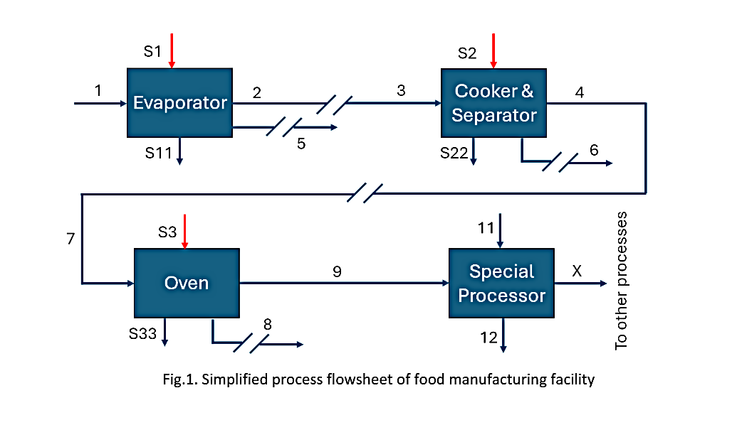
Fig.1. Simplified process flowsheet of food manufacturing facility.

 

Note on storage and system boundaries:

Because the two sub-processes occur at different times, direct process-to-process heat exchange between their streams is not possible without thermal storage. If storage is introduced: 

• Production surplus heat at time slice A can be stored at high temperature (e.g., 80 °C) and later discharged to preheat time slice B cold streams. 

• The size of the tank depends on the portion of hot utility demand of sub-process B to be offset, the temperature swing, and the duration of the sub-process B. 

 

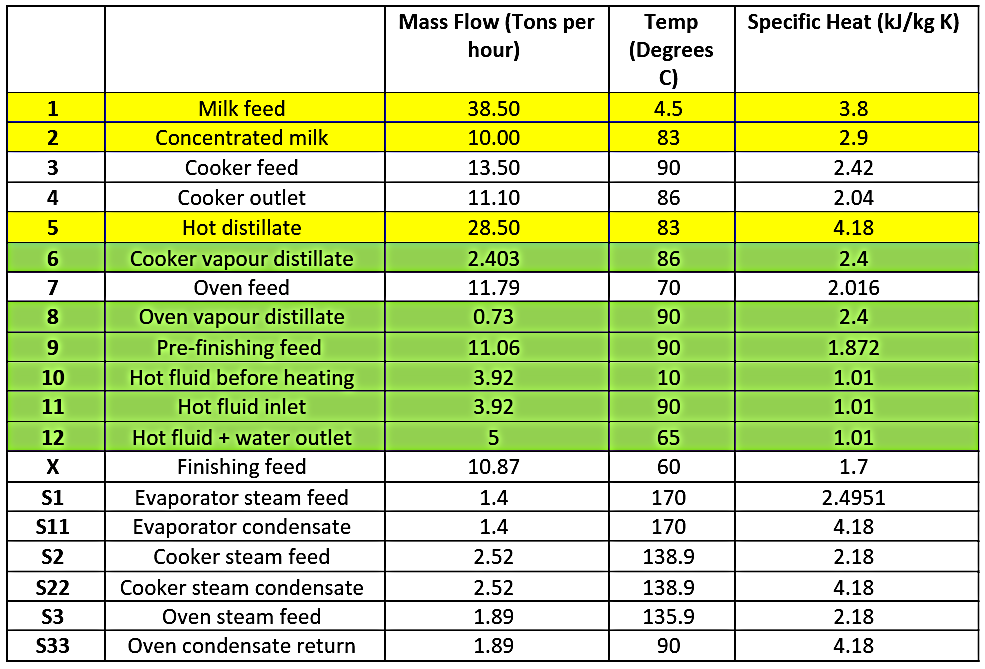
Table 1. Process stream data corresponding to flowsheet of Fig. 1. Yellow-highlighted sections represent processes available at time slice A, while green-highlighted sections are processes available at time slice B.

 

Appendix B: Suggested marking rubric (Editable):

Adopter note: The rubric below is a suggested template. Instructors may adjust criteria language, weightings and band thresholds to align with local policies and learning outcomes. No marks depend on running software. 

1) Interpretation of Simulation Outputs — 25% 

• A (Excellent): Reads curves/tables correctly; uses QHU/QCU/QREC, COP, CAPEX/OPEX/CO₂, payback figures accurately; draws clear, defensible trade-offs. 

• B (Good): Mostly accurate; links numbers to decisions with some insight. 

• C (Adequate): Mixed accuracy; limited or generic trade-off discussion. 

• D/F (Weak): Frequent misreads; cherry-picks or contradicts generated data. 

2) Systems Thinking & Scenario Analysis — 30% 

• A: Clear CLD with at least one reinforcing and one balancing loop; leverage points identified; scenarios coherent; MCDA with explicit criteria, weights, and justified ranking; uncertainty acknowledged. 

• B: Reasonable CLD; scenarios sound; MCDA present with partial justification. 

• C: Superficial CLD; scenarios/MCDA incomplete or weakly reasoned. 

• D/F: Little or no systems view; scenarios/MCDA absent or not meaningful. 

3) Stakeholder & Implementation Insight — 20% 

• A: Balanced perspectives (operations, finance, environment, policy); realistic risks/constraints (e.g., fouling, downtime, grid-carbon variability, funding) with feasible mitigations. 

• B: Multiple perspectives; several relevant risks noted. 

• C: Narrow view; risks generic or unconnected to context. 

• D/F: Stakeholders and practicalities largely ignored. 

4) Decision Quality & Justification — 15% 

• A: Clear recommendation grounded in evidence; includes one sensible “what-if” sensitivity; states assumptions/limits explicitly. 

• B: Recommendation mostly supported; partial sensitivity/assumptions. 

• C: Vague or weakly justified; little sensitivity analysis. 

• D/F: No defensible recommendation; reasoning unclear. 

5) Communication & Presentation — 10% 

• A: Concise, well-structured portfolio; labelled figures; readable MCDA; legible diagrams; professional formatting. 

• B: Generally clear; minor layout/label issues. 

• C: Uneven structure/clarity; some labels missing. 

• D/F: Disorganised; difficult to follow. 

 

References:

• Atuonwu, J.C. (2025). A Simulation Tool for Pinch Analysis and Heat Exchanger/Heat Pump Integration in Industrial Processes: Development and Application in Challenge-based Learning. Education for Chemical Engineers 52, 141-150. 

• The Government Office for Science (2022). Systems Thinking Case Study Bank. https://assets.publishing.service.gov.uk/media/6290d252e90e070396c9f66c/GO-Science_Systems_Thinking_Case_Study_Bank_2022_v.1.pdf (Accessed 06/08/2025). 

• Energy Catapult (2025). Systems thinking in the energy system. A primer to a complex world. (Accessed 06/08/2025) https://esc-production-2021.s3.eu-west-2.amazonaws.com/2022/03/Systems-thinking-in-the-energy-system.pdf. 

• HM Government (2021). UK Industrial Decarbonisation Strategy. https://assets.publishing.service.gov.uk/media/6051cd04e90e07527f645f1e/Industrial_Decarbonisation_Strategy_March_2021.pdf (Accessed 06/08/2025). 

• Oh, X.B., Rozali, N.E.M., Liew, P.Y., Klemes, J.J. (2021). Design of integrated energy- water systems using Pinch Analysis: a nexus study of energy-water-carbon emissions. Journal of Cleaner Production 322, 129092. 

• NMITE (2025). Researcher Develops Cutting-Edge Simulation Tool for Industrial Decarbonisation. https://nmite.ac.uk/NMITEXChange/the-NMITEXChange-feed/nmite-researcher-develops-cutting-edge-simulation-tool-industrial-decarbonisation (Accessed 07/08/2025). 

• IPECA (2022). Pinch Analysis.  https://www.ipieca.org/resources/energy-efficiency-compendium/pinch-analysis-2022 (Accessed 11/08/2025).

• Rosenow, J., Arpagaus, C., Lechtenböhmer, S.,Oxenaar, S., Pusceddu, E. (2025). The heat is on: Policy solutions for industrial electrification. Energy Research & Social Science 127, 104227. 

• SankeyMATIC (2025). Online Interactive Tool for drawing Sankey Diagrams. (Accessed 12/08/2025) https://sankeymatic.com/ 

• Bale, C.S.E., Varga, L., Foxon, T.J. (2015).  Energy and complexity: New ways forward. Applied Energy 138, 150-159. 

• Atuonwu, J.C. (2025). Proprietary Simulator for Pinch Analysis & Heat Integration. Private reviewer access available on request (demo video or temporary login).  

 

Any views, thoughts, and opinions expressed herein are solely that of the author(s) and do not necessarily reflect the views, opinions, policies, or position of the Engineering Professors’ Council or the Toolkit sponsors and supporters.